

Introduction
The use of RF pulses to detect objects in three dimensions started in the early 1900s. Initial applications focused on military requirements, specifically detection of ships and aircraft. Today, radar is used in a wide range of military, commercial and research applications including tracking aircraft, monitoring the weather and detecting the speed of anything from a tennis ball to a car. The basic principle of radar remains unchanged, with a short burst of RF energy being transmitted and then a receiver waiting to detect any of that energy that has bounced back from a distant object.
Once installed, many radars are expected to run uninterrupted for decades of service. To ensure that their performance does not degrade over time, it is necessary to measure their key performance metrics at regular intervals. One of the prime areas of performance that is monitored is the characteristics of the transmitted RF pulses. The IEEE has published specifications for how the critical parameters of pulses should be measured, “IEEE Std 181-2011, Standard for Transitions, Pulses and Related Waveforms”. This standard specifies precisely what parameters need to be measured and how those measurements should be calculated.


The Field Master Pro MS2090A with option 0421 pulse analyzer displays the full pulse characteristics and provides detailed numeric results for all the common radar parameters. This application note highlights its use in field measurements of airport surveillance radar and weather radar.
Airport Surveillance Radar
In 1998 the United States Federal Aviation Administration (FAA) introduced a new airport surveillance radar called ASR-11 that tracks aircraft movement and additionally provides some weather information. There are now over 400 of these radars deployed across the USA.
| ASR-11 Airport Surveillance Radar | |
| Manufacturer | Raytheon |
| Frequency | 2.7 to 2.9 GHz |
| Range | 60 Miles (~97 km) |
| Peak Power | 25 kW |
| Pulse Width | 1 µs to 80 µs |
| Pulse Repetition Frequency | ~ 1 ms |
| Rotation Rate | 12.5 RPM |
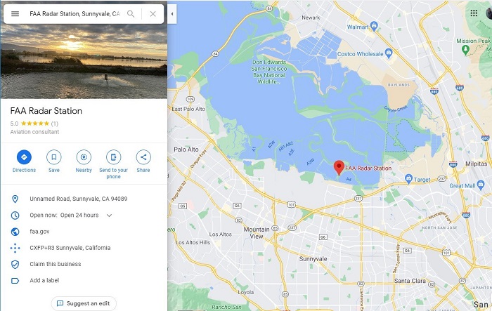
The high peak power from these radars makes them very easy to detect miles from their location. For example, the FAA radar covering the San Francisco Bay Area is located at the south end of the bay as seen in the map figure 1.
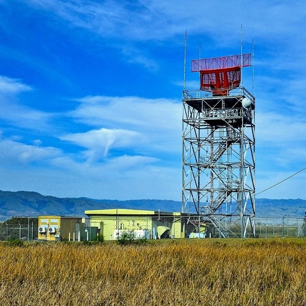
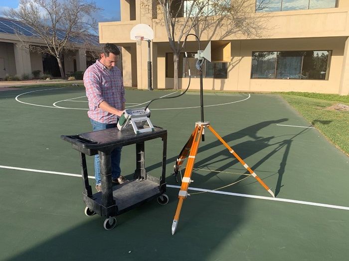
This specific radar transmits at 2.875 GHz. Mounting a 2 to 4 GHz waveguide antenna on a tripod at a distance of around 50 kilometers, the radar pulses are easily detectable (figure 3).
Due to the rotation of the radar antenna the pulses are only directed at the receiving analyzer approximately every 5 seconds as seen in figure 4.
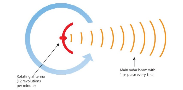
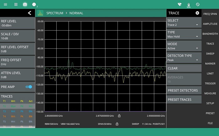
Figure 5 shows that due to the short duration of the pulses and the rotation of the transmitting antenna, a spectrum analyzer in frequency sweep mode does not capture the signal, even with trace maximum hold applied.
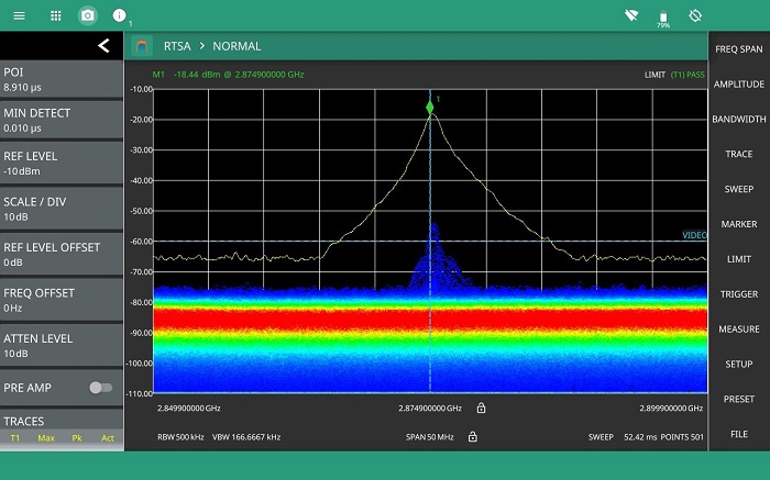
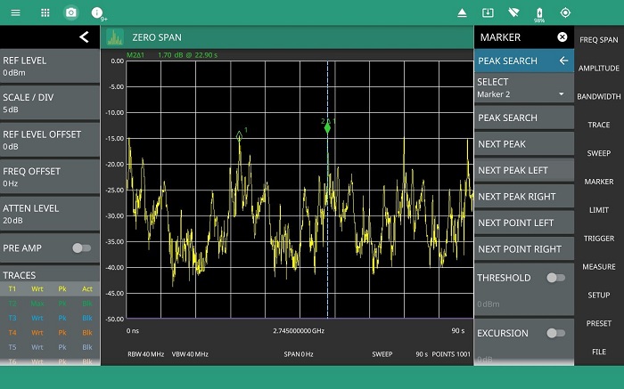
By switching the analyzer mode to view the signal with the RTSA, one can see the radar signal is always captured (figure 6). The RTSA continuously displays the radar pulse power which appears to rise and fall as the rotating antenna points towards the waveguide horn antenna connected to the Field Master Pro MS2090A and then rotates away from it. This has the effect of displaying a power spectrum density that appears to “breath”. Use of a maximum hold trace provides a good indication of the current signal level relative to the maximum condition (figure 7).

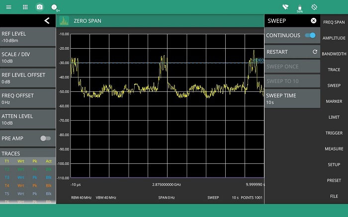
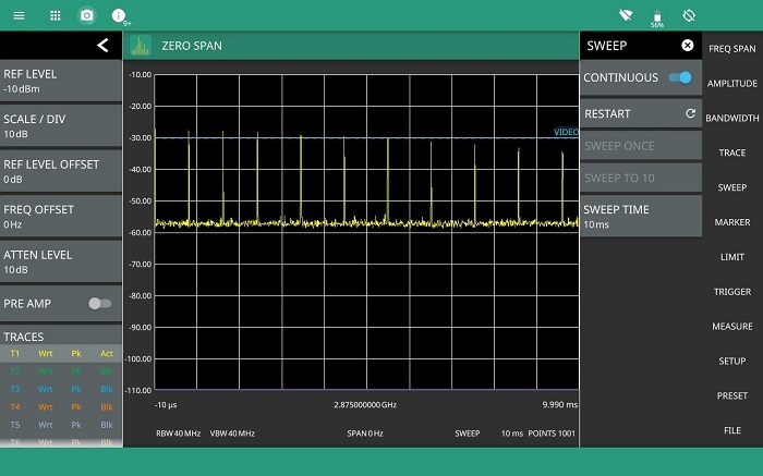
To view the pulses in time domain, the spectrum analyzer is put into zero span mode. This fixes the frequency of the analyzer input and displays power against time on the display. Initially, it is interest- ing to set a long time span so that the radar transmitter pulses can be seen. Figure 8 shows the groups of pulses displayed with a nominally 5 second duty cycle as the radar transmitter rotates. In this case, each of the bursts of RF energy contains many individual 1 µs pulses.
Although measurements on the pulses can be made in zero span mode by positioning markers on the trace, this does not have the accuracy or measurement traceability provided by option 0421 pulse analyzer.
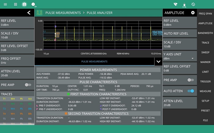
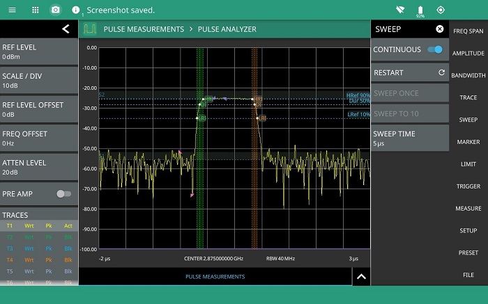
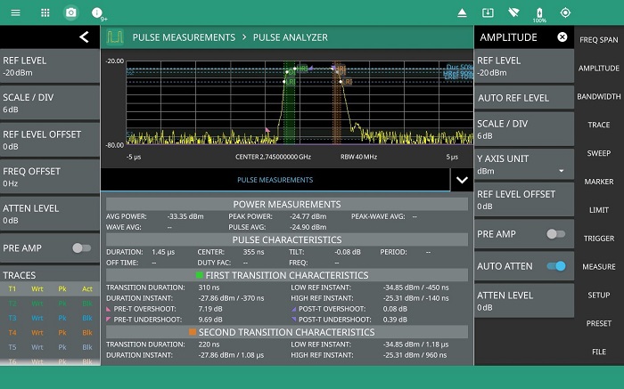
Enabling the pulse analyzer option provides measurements on pulses and pulse streams in full compliance with the IEEE standard. For measurements of pulse repetition frequency, duty cycle and off time, at least two pulses must be captured and displayed, typically it is better to capture more (figure 11). Depending on the pulse train and individual pulse characteristics, it may not be possible to perform all measurements such as rise time in the same span.
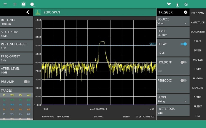
Set the video trigger level and pre trigger delay to display a stable stream of pulses on the instrument display. The pulse analyzer option automatically populates all the measurements that can be performed on the captured data, no additional set up is required.
Reduce the sweep time to display a single pulse. Vertical marker lines are automatically placed on the 10% and 90% linear power points for rising and falling edges as well as horizontal markers for the 50% reference level used to measure pulse duration. The values IEEE default values can be manually overridden if required. (Details of the IEEE measurement can be found in the appendix.)
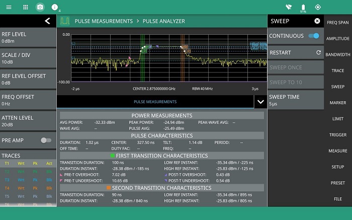
Figure 13 shows a full screen view mode is available for a more detailed view of a single pulse.
With the Field Master Pro MS2090A pulse analyzer option, field measurements of airport surveillance radars can be completed accurately and quickly without interrupting operation.
Weather Radar
Another common application of radar is to monitor weather conditions, including rainfall, storms, and snow. Weather radars can be ground based for actively tracking rainfall and storms or satellite based for wider area monitoring. In the USA a network of over 150 ground based weather radars is operated by the national weather center. Known as the Next Generation Weather Radar (NEXRAD) system, the first radars were deployed and operated in the 1990’s and the system is under continual enhancement.
| WSR-88D National Weather Radar | |
| Prime Contractor | Unisys |
| Frequency | 2.7 to 3.0 GHz |
| Range | 90 to 150 Miles (~145 to 240 km) |
| Peak Power | 700 kW |
| Pulse Width | ~ 1 µs to 5 µs |
| Pulse Repetition Frequency | ~ 1 ms |
| Rotation Rate | 3 RPM |
The weather radar characteristics are similar to the airport surveillance radars. Both use the same frequency band and high power pulses. Frequency planning is important to ensure there is no interference between the technologies. The weather radar that covers the San Francisco Bay Area is located on Mount Umunhum about 20 miles south of San Jose.
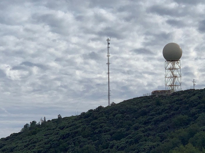
The Mount Umunhum weather radar transmits at 2.745 GHz and the antenna rotates about 3 times a minute (figure 15). The pulse train varies depending on the conditions at the time. Dense rain will reflect more power and reduces the range.
The test set up for this radar is similar to that described previously for the airport surveillance radar. A waveguide horn antenna connected to the Field Master Pro MS2090A and pointed in the direction of the radar enables measurements to be made many miles from the radar location.
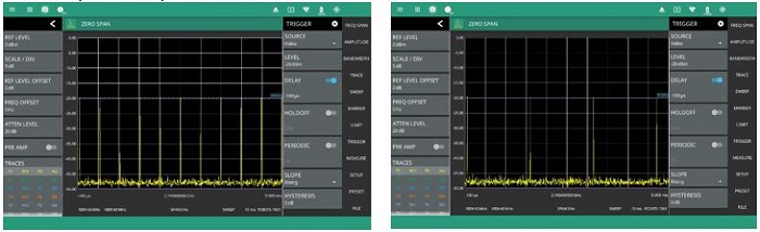
Analyzing the pulse trains in zero span mode highlights the change in pulse repetition frequency used by the radar in different modes to analyze changes in atmospheric conditions. Figure 16 shows the difference in two separate captured views
The pulse analyzer option again provides quick detailed analysis of the pulse train and individual pulse characteristics that can be seen in figure 17.
Summary
The Field Master Pro MS2090A pulse analyzer option provides a powerful test solution to measurement pulsed radar signals in the field. The wide measurement bandwidth supports rise time measurements as fast as 30 ns. Coupled with IEEE compliant pulse measurements, routine testing of radars for maintenance or troubleshooting applications is possible in a way that was previously restricted to the lab and can be accomplished in the field.
Appendix: Summary of Pulse Measurements Supported
Pulse Measurements
Finding the High/Low Reference Levels Using the Histogram Algorithm
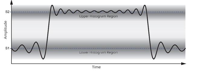
When the pulse level type is set to AUTO a histogram algorithm method is used for determining the high and low state levels as described in the IEEE Standard for Pulses, Transitions, and Related Waveforms (181-2011), Section 5.2.1. The trace data is taken as input and the amplitudes are operated on in terms of dBm units. The trace data is converted into a histogram where the number of bins is determined by a fixed bin width of 0.01 across the total range of values in the trace data (trace max to trace min). In other words, each trace point amplitude results in an incremented “count” in the histogram bin that corresponds to the amplitude range in which that amplitude falls. To find the high and low state levels, the resulting histogram is split into an “upper” and “lower” histogram where the former consists of all the bins that correspond to the upper 50% range of amplitudes, and the latter the lower 50% range. Then the high state is determined to be the mode of the upper histogram, i.e. the amplitude corresponding to the histogram bin with the highest count. The low state is similarly determined to be the mode of the lower histogram.
If the count of either mode is not greater than at least 1% of the total number of points in the trace data input, then the histogram is recreated using a bin width that is ten times larger. This process of regenerating the histogram with larger a bin width is repeated until the mode of the histogram is at least 1% of the total number of points. This means that the best case resolution of the resulting high state and low state is 0.01 dBm (the starting bin width), and depending on how much the state levels fluctuate, the resolution can fall back to 0.1 dBm, 1 dBm, and so on.
When the pulse level type is set to USER, the user determines the high and low state levels and enters the level using the USER TOP (S2) and USER BOTTOM (S1) settings.
Finding the Reference Level Instants
Instants are a specific time value within a waveform time duration. They are typically referenced relative to the initial instant of the waveform. The following sections describe how the pulse measurements are determined
Finding the Transitions
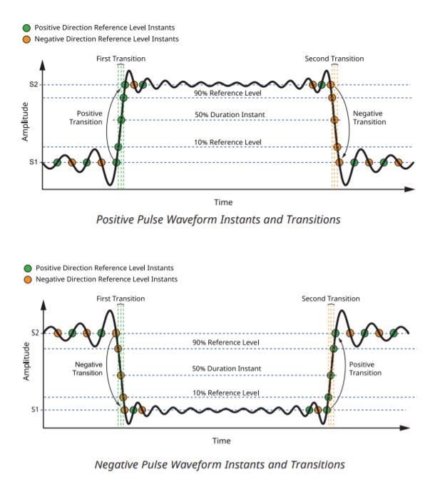
Transitions are contiguous regions of a waveform that connect, either directly or via intervening transients, two state occurrences that are consecutive in time but are occurrences of different states. To find the transition, begin with a filtered list of reference level instants that contain only those that cross the low or high reference levels. Each reference level instant in the list has a corresponding index and direction (e.g. the trace index immediately before the amplitude crossing the reference level, and direction indicating whether the trace crosses from above to below the reference level or vice versa).
This filtered list of instants is sorted in ascending index order. Then all positive and negative transitions (between the high/low reference levels) are found by searching for consecutive instants in the filtered list that both have the same direction. The waveform is defined to be in the “high state” if it exceeds the 90% reference level and in the “low state” if it drops below the 10% reference level. This is the chosen alternative rather than using the state upper/lower boundaries (which the IEEE standard says is optional).
Finding Pulse Duration and Period
The pulse duration is determined by using the positive and negative transitions as describe above to check if it is a valid pulse. If so, then any pulse duration reference levels (50%) are verified to exist within the positive/negative transition. This reference level determines the starting and ending period of the pulse. The duration is just the difference between the ending point and the starting point. The pulse period also first determines that we have a valid pulse from the positive and negative transitions. Unlike the pulse duration measurement, the pulse period must have the pulse repeat, or a pulse train, to have a measurement. There should be at least 3 transitions in the 50% reference level to produce a valid measurement. The period is the distance between the starting level of the first pulse and the starting level for the second pulse.
Finding the Wave Average
The wave average is determined by averaging the power levels of all points within all complete periods that are available on the trace. To determine where to start and stop, the number of transitions is used to determine if there is at least one full period. The system returns “nan” if there is not a full period. Otherwise, the starting point for this measurement is the beginning of the first transition and the end point is the beginning of the transition of the last full period.
For instance, a trace with six transitions has some quantity of points before the first transition followed by two full periods, then followed by less than one full period. Once the start and end of all the complete periods have been found, all points between them are summed together and divided by the total number of points used in the measurement.
The trace average is the exponential average of all the points in the trace. Unlike the wave average, it is not constrained to full pulses.
Finding the Pulse Average
The pulse average is the average of the points in the high state of the pulse (typically those points above the 90% reference line). This only applies to positive pulses. If there is no positive pulse, then no measurement is returned.
Finding the Pulse Center Instant and Repetition Frequency
The Pulse repetition frequency is determined from the inverse of the pulse period (1/pulse period) as a frequency value. The pulse center instant is determine by taking the pulse duration (50%) start time and adding the pulse duration midpoint, which is one-half of the pulse duration (pulse duration/2).
Finding the Pulse Peak
The pulse peak is the maximum value in a waveform after a positive transition. If there is no positive transition, the peak amplitude of the overall waveform is returned.
Finding the Pulse Tilt
The pulse tilt measures the distortion of a waveform state where the overall slope of the state is essentially constant and other than zero. The slope may be of either polarity and is calculated for either negative or positive pulses. A complete pulse (with at least two transitions) is needed to ensure that there is a waveform state for which tilt can be measured. If there is enough trace data within the waveform state, the first and last 25% of samples where overshoot distortion is most likely to occur is removed. The slope of the remaining 50% of state trace data is then calculated using the least squares method, and the tilt is calculated by multiplying the slope by the number of trace points in the state.
Finding the Wave Amplitude
The wave amplitude is found by subtracting the amplitude of the lower state level from the amplitude of the upper state level in dB units.
Finding the Peak to Wave Average
The peak to wave average is found by subtracting the wave average from the pulse peak in terms of dB. This requires the wave average to have a valid value, so there must be at least one full period for a measurement.
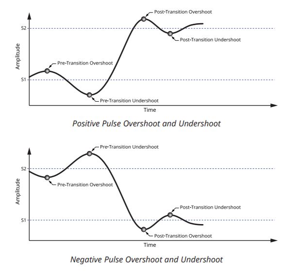
Finding the Pre- and Post-Transition Aberration Region
The pre-transition aberration region is determined to be the region of the trace before the last state crossing before the first transition, and with a width equal to three times the duration of the first transition. It is upper bounded by the available trace data before the transition. The post-transition aberration region is the region beginning at the first state crossing past the first transition, and ending at three times the transition duration or at the beginning of the next transition, whichever comes first.
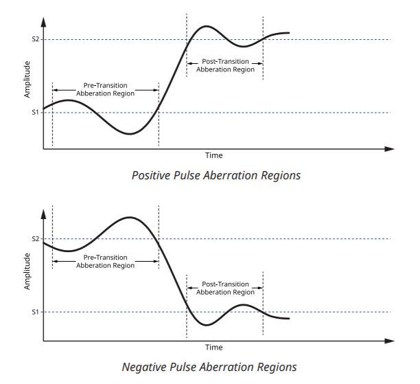
Finding the Overshoot and Undershoot of Each Aberration Region
The overshoot and undershoot of each region are calculated by taking the difference between the maximum and minimum trace value of each aberration region and the local state level. Local state level being (Low = pre-transition → High = post-transition) in a positive transition, and (High = pre-transition → Low = post-transition) in a negative transition