


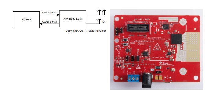
 application using the AWR1642 evaluation module (EVM). This design allows)
Description
The TIDEP-0092 provides a foundation for a short range radar (SRR) application using the AWR1642 evaluation module (EVM). This design allows the user to estimate and track the position (in the azimuthal plane) and the velocity of objects in its field of view up to 80 m.


Features
- Single-Chip FMCW Radio Detection and Ranging (RADAR) for SRR Applications
- Detect Objects (Such as Cars and Trucks) up to
- 80-m Away With Range Resolution of 35 cm;
- Objects 20-m Away Detectable With Resolution of 4.3 cm
- Clustering and Tracking on Detected Outputs
- Antenna Field of View ±60º With Angular Resolution of Approximately 15º
- Source Code for Fast Fourier Transform ( FFT )
Processing and Detection Provided by mmWave
- Software Development Kit ( SDK )
- AWR1642 Demonstrates Design
- Radar Front End and Detection Configuration Fully Explained
Applications
- Lane Change Assist (LCA)
- Autonomous Parking
- Cross Traffic Alert (CTA)
- Blind Spot Detection (BSD)
1 System Description
Autonomous control of a vehicle provides quality-of-life and safety benefits in addition to making the relatively mundane act of driving safer and less difficult. The quality-of-life features include the ability of a vehicle to park itself or to determine whether a lane change is possible and provide features like automatic cruise control—where a vehicle maintains a constant distance with respect to the car ahead of it, essentially tracking the velocity of the car in front of it. Autonomous breaking and collision avoidance are safety features that prevent accidents caused by driver inattention. These features work by observing the area in front of a car and alerting the autonomous driving subsystems if obstacles are observed that are likely to hit the car. Implementing these technologies require a variety of sensors to detect obstacles in the environment and track their velocities and positions over time.
1.1 Why Radar?
Frequency-modulated continuous-wave (FMCW) radars allow the accurate measurement of distances and relative velocities of obstacles and other vehicles; therefore, radars are useful for autonomous vehicular applications (such as parking assist and lane change assist) and car safety applications ( autonomous breaking and collision avoidance). An important advantage of radars over camera and light-detection-andranging (LIDAR)-based systems is that radars are relatively immune to environmental conditions (such as the effects of rain, dust, and smoke). Because FMCW radars transmit a specific signal (called a chirp) and process the reflections, they can work in complete darkness and also bright daylight (radars are not affected by glare). When compared with ultrasound, radars typically have a much longer range and much faster time of transit for their signals.
1.2 TI SRR Design
The TIDEP-0092 is an introductory application that is configured for short range applications (that is to detect as many as 200 objects up to a distance of 80 m (260 feet) and track as many as 24 of them travelling as fast as 90 kph, which is approximately 55 mph). In the short range application, the AWR1642 sensor is configured as a multi-mode radar, which means that it can simultaneously track objects at 80 m while generating a rich point cloud of objects at 20 m, so that approaching vehicles and closer small objects can be detected at the same time. This reference design can be used as a starting point to design a standalone sensor for a variety of SRR automotive applications. A range of more than 80 m can be achieved with the design of an antenna with higher gain than the one included in the AWR1642.
1.3 Key System Specifications
This reference design has two sets of specifications because the radar is used as a multi-mode radar. The first specification is for the short range radar (SRR), which has a range of 80 m. The second specification is for the ultra-short-range radar (USRR), which has an effective range of only 20 m.
Table 1. Key System Specifications
| PARAMETER | SPECIFICATIONS | DETAILS |
| Maximum range | 80 m (SRR), 2 0m (USRR) | This represents the maximum distance that the radar can detect an object representing an RCS of approximately 10 m2 . |
| Range resolution | 36.6 cm (SRR), 4.3 cm ( USRR ) | Range resolution is the ability of a radar system to distinguish between two or more targets on the same bearing but at different ranges. |
| Maximum velocity | 90 kph (SRR), 36 kph ( USRR ) | This is the native maximum velocity obtained using a two-dimensional FFT on the frame data. This specification will be improved over time by showing how higher-level algorithms can extend the maximum measurable velocity beyond this limit. |
| Velocity resolution | 0.52 m/s (SRR), 0.32 m/s (USRR) | This parameter represents the capability of the radar sensor to distinguish between two or more objects at the same range but moving with different velocities. |
2 System Overview
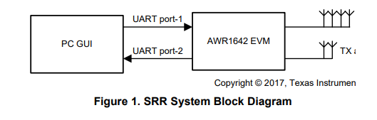
2.1 Block Diagram
2.2 Highlighted Products
2.2.1 AWR1642 Single-Chip Radar Solution
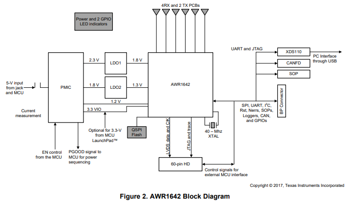
The AWR1642 is an integrated single-chip, frequency modulated continuous wave (FMCW) sensor capable of operation in the 76 to 81 GHz frequency band. The device is built with TI’s low-power, 45- nm RFCMOS processor and enables unprecedented levels of analog and digital integration in an extremely small form factor. The device has four receivers and two transmitters with a closed-loop phase-locked loop (PLL) for precise and linear chirp synthesis. The sensor includes a built-in radio processor (BIST) for RF calibration and safety monitoring. Based on complex baseband architecture, the sensor device supports an IF bandwidth of 5 MHz with reconfigurable output sampling rates. The presence of ARM Cortex R4F and Texas Instruments C674x Digital Signal Processor (DSP) (fixed and floating point) along with 1.5 MB of on-chip RAM enables high-level algorithm development.
2.2.2 AWR1642 Features
The AWR1642 has the following features:
- AWR1642 radar device
- Power management circuit to provide all the required supply rails from a single 5-V input
- Two onboard TX antennas and four RX antennas
- Onboard XDS110 that provides a JTAG interface, UART1 for loading the radar configuration on the
AWR1642 device, and UART2 to send the object data back to the PC
2.3 System Design Theory—Chirp Configuration
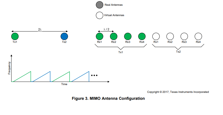
2.3.1 Antenna Configuration
The TIDEP-0092 uses four receivers and the two transmitters in two different chirp configurations. The first configuration (SRR) uses a simple non-multiple-input and multiple-output (MIMO) configuration with only TX1 transmitting. The second configuration (USRR) uses a time division multiplexed MIMO configuration (that is, alternate chirps in a frame transmit on TX1 and TX2 respectively.). The MIMO configuration synthesizes an array of eight virtual RX antennas, as shown in Figure 3. This technique improves the angle resolution by a factor of two (compared to a single TX configuration).
 2.3.2 Chirp Configuration and System Performance
To achieve the specific SRR use case with a visibility range of approximately 80 m and memory availability of AWR1642, the chirp configuration in Table 2 is used.
Table 2. Chirp Configuration
| PARAMETER | SPECIFICATIONS |
| Idle time (µs) | 3 (SRR), 7 ( USRR ) |
| ADC start time (µs) | 3 (SRR), 5 ( USRR ) |
| Ramp end time (µs) | 56 (SRR), 87.3 ( USRR ) |
| Number of ADC samples | 256 (SRR), 512 ( USRR ) |
| Frequency slope (MHz/µs) | 8 (SRR), 42 ( USRR ) |
| ADC sampling frequency (ksps) | 5000 (SRR), 6250 ( USRR ) |
| MIMO (1→yes) | 0 (SRR), 1 ( USRR ) |
| Number of chirps per profile | 128 (SRR), 64 ( USRR ) |
| Effective chirp time (usec) | 51 (SRR), 82 ( USRR ) |
| Bandwidth (MHz) | 409 (SRR), 3456 ( USRR ) |
| Frame length (ms) | 7.3 (SRR), 6.03 ( USRR ) |
| Memory requirements (KB) | 512 (SRR and USRR) |
The Table 2 configuration is selected to achieve the system performance shown in Table 3. The primary goal was to achieve a maximum distance of about 80 m. Note that the product of the frequency slope and the maximum distance is limited by the available IF bandwidth (6.25 MHz for the AWR1642). Thus, a maximum distance of 85 m locks down the frequency slope of the chirp to about 8 MHz/µs. The choice of the chirp periodicity is a trade-off between range resolution and maximum velocity. This design uses a range-resolution of about 0.3 m, which leaves a native maximum velocity of about 55 kph . Through high-level algorithms, the maximum unambiguous velocity that can be detected is 90 kph.
A larger maximum distance translates to a lower range resolution (due to limitations on both the L3 memory and the IF bandwidth). A useful technique to work around this trade-off is to have multiple configurations with each tailored for a specific viewing range. For example, it is typical to have the SRR radar alternate between two modes: a low-resolution mode targeting a larger maximum distance (such as 85 m with 0.3-m resolution) and a high-resolution mode targeting a shorter distance (such as 20 m with a 4-cm resolution). This multi-mode capability is implemented in the current SRR design.
Though not implemented in the current SRR design, note that there are several approaches that can improve the maximum detectable velocity several multiples beyond this native maximum.
Table 3. System Performance Parameters
| PARAMETER | SPECIFICATIONS |
| Range resolution (m) | 0.36 (SRR), 0.043 ( USRR ) |
| Maximum distance (m) | 80 (SRR), 20 ( USRR ) |
| Native maximum velocity (kph) | 90 (SRR), 36 ( USRR ) |
2.3.3 Configuration Profile
To meet the requirements for both USRR and SRR use cases, this reference design makes use of the ‘advanced frame config’ application programming interface (API) of the AWR1642 device. This API allows the construction of a frame consisting of multiple subframes, with each subframe being tuned to a particular application. Such a design is referred to as multi-mode radar. Each of these subframes tune to one application. In the case of the SRR configuration, use two subframes. One subframe is dedicated to the USRR context and the other to the SRR context.
The frame configuration utilizes the ‘advanced frame config’ API to generate two separate subframes: the SRR subframe and the USRR subframe (with the subframes being named after their principle design requirement). Figure 4 shows the frame configuration.
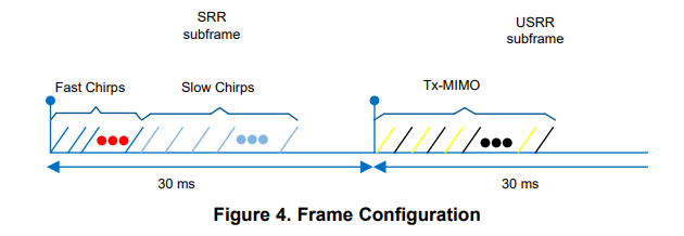
- SRR subframe
This subframe consists of two kinds of chirps (fast chirps and slow chirps). Both fast and slow chirps have the same slope; however, the slow chirp has a slightly higher ‘chirp repeat periodicity’ than the fast chirp. As a result, the slow chirps (when processed after 2D fast-Fourier transform (FFT)) have a lower maximum unambiguous velocity as compared to the fast chirps. Note that the fast and slow chirps do not alternate; instead, the fast chirp is repeated a certain number of times, followed by the slow chirp, which is again repeated an equal number of times.
The purpose of this chirp design is to use the two separate estimations of target velocity from the ‘fast chirp’ and the ‘slow chirp’ along with the ‘Chinese remainder theorem’ to generate a consistent velocity estimate with a much higher max-velocity limit.
- USRR subframe
This subframe consists of two alternating chirps. Each chirp utilizes one of the two Txs available on the AWR1642 device. Combined processing of this subframe allows the generation of a virtual Rx array of eight Rx antennas, which consequently has better angular resolution (approximately 14.3°) than the 4 Rx antenna array.
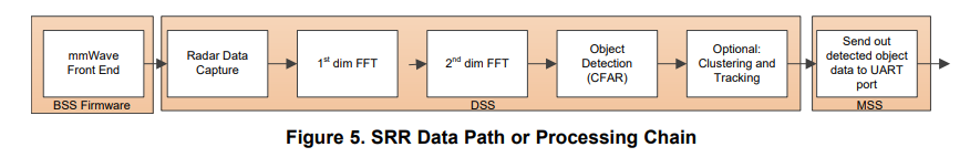
2.3.4 Data Path
The block diagram in Figure 5 shows the processing data part to the SRR application.
2.3.5 Chirp Timing
Figure 6 shows the timing of the chirps and subsequent processing in the system.
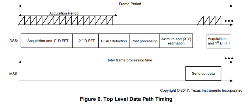
Figure 6 shows the data path processing, which is described as follows.
- The RF front end is configured by the BIST subsystem (BSS). The raw data obtained from the various front end channels is taken by the C67x DSP subsystem (DSS) for processing.
- Processing during the chirps as seen in Figure 6 consists of:
- 1D (range) FFT processing performed by the C674x that takes input from multiple receive antennae from the ADC buffer for every chirp (corresponding to the chirping pattern on the transmit antennae)
- Transferring transposed output into the L3 RAM by enhanced direct memory access ( eDMA )
- Processing during the idle or cool down period of the RF circuitry following the chirps until the next chirping period, shown as Inter frame processing time in Figure 6. This processing consists of:
- 2D (velocity) FFT processing performed by C674x that takes input from 1D output in L3 RAM and performs FFT to give a (range, velocity) matrix in the L3 RAM. The processing also includes the CFAR detection in Doppler direction. CFAR detection in range direction uses the mmWave library.
- Peak grouping (for both Doppler and range) for the SRR subframe and Doppler for the USRR subframe
- Direction of arrival (azimuth) estimation to map the X-Y location of object
- Additional pruning based on the SNR and the 2D-FFT magnitude of the object to avoid ground clutter
- Clustering of detected objects using the dBScan algorithm for both SRR and USRR – Tracking of clusters using an extended Kalman filter for the SRR
Clustering
Clustering is performed using the dBscan algorithm [9] which is applied on the detected objects of both the SRR and the USRR subframes. The output of the clustering algorithm is the mean location of a cluster and its dimensions (assuming the cluster is a rectangle).
For the USRR subframe, the clustering output is sent as is to the graphical user interface (GUI). USRR clusters allow the grouping of dense point clouds to rectangles. In cross-traffic scenarios, these clusters can be used to identify vehicles crossing the field of vision (FoV) of the radar.
For the SRR algorithm, the clustering output is used as the basis for the input to the tracking algorithm. The strongest object in the cluster is provided as the representative object to the tracking algorithm. The intention here is essentially reduce the number of objects provided to the tracking algorithm and introduce hysteresis, so that the trackers only track strong reflectors, and do not switch between adjacent reflectors.
Tracking
The tracker is a fairly standard Extended Kalman Filter (EKF with four states [x, y, vx, vv] and three inputs [r, v, sin(θ)] or range, relative velocity, and sin of the azimuth). Compute the associated variances for the inputs using the associated signal-to-noise ratio (SNR) for each input. Use the Cramer-Rao lower bound (CRLB) formula for frequency variance to convert the SNR to a variance. The variance is lower-bounded by the resolution of the various inputs.
While the tracker is quite standard for an EKF, there are two functions in the tracker that can be modified based on the requirements. The first is the ‘track initialization function’ (initNewTracker), where the initial parameters of the track are populated. In the SRR design, the assumption is that the velocity of the object is only along the longitudinal axis. In other words, a vehicle with a relative velocity v is assumed to be travelling towards the radar with vx = 0 , and vv = v , which works well in long-range highway traffic, but is less effective in cross-traffic situations.
The second function is the ‘data association function’ (isTargetWithinDataAssociationThresh), which associates new measurements with existing tracks. Association essentially requires assumptions on the movement of objects in the scene, including maximum velocities, directions of motion, accelerations when close to the radar, and so forth.
eDMA configuration
Large-scale data movement between memories is accomplished in both the out-of-box (OOB) demo of the mmWave SDK and the SRR using the eDMA. Using the eDMA is more efficient than using the processor to move data because, while the data movement is being completed, the DSP can continue to process data. The major data transfers necessary in the OOB demo include:
- Movement of ADC data from the ADC buffer to the DSP L2/L1 memory
- Movement of 1D-FFT data from the DSP L1/L2 memory to the L3 memory to form the ‘radarcube matrix’
- Fetching the 1D-FFT data from L3 to do 2D FFT
- Movement of the ‘sumAbs’ array from the L2/L1 to L3 to form the detection matrix
- Movement of slices of the detection matrix in L3 to L2/L1 to do detection
- Movement of 1D-FFT data from L3 to do angle estimation (after 2 D-DFT )
Most of the eDMAs work on a ping-pong buffer, which means that as the ping buffer is being filled, the pong buffer can be used by the DSP for processing. The eDMA configuration in the SRR demo is very similar to the eDMA configuration on the OOB demo. The differences relate to the processing of two different subframes, and the processing of the SRR subframe.
In order to process the two different subframes, the SRR demo simply doubles the number of number of assigned eDMAs so that each subframe has its own subset of eDMAs to perform the necessary transfers. This method will not scale as the number of subframes increase, and it is recommended that if more than 3 subframes are to be programmed, then one should reprogram the eDMAs after a frame is processed ( as is done in the OOB demo).
To process the ‘max velocity enhancement’ subframe, the eDMAs listed as 2, 3, and 6 must be changed, so that they transfer twice as many chirps.
Memory allocation
The AWR1642 (PG 2.0) has the following memories on the DSP.
- L3 RAM of 768kB (PG 1.0 has 640 kB)
- L2 RAM of 256 kB
- L1 RAM of 32kB each
The R4F has 512kB of code and data RAM. In the SRR design, the R4F is used only for configuration and for the universal asynchronous receiver/transmitter (UART) or loop-voltage differential-signaling ( LVDS ) communication. The RF4 memory consumption and allocation are not of any concern to the design. The DSP, therefore, is the main consumer of memory, for which the allocations are discussed below.
Of the 32KB for the available L1P RAM and L1D RAM, half (16kB) of the L1P RAM and half (16kB) of the L1D RAM are reserved for code and data storage. The remaining are used as cache. The code stored in L1P is typically algorithms like the FFTs or the CFAR, or some of the kernels of more complex algorithms like clustering and tracking. Storing these in L1 allows faster execution of these kernels as well as saving some space (in the case of this design, approximately 16kB) in the remaining memories. The L1D is used as fast RAM for certain commonly-used buffers.
L2 RAM is used for code-storage as well as scratch buffers and state information for the different algorithms, as well as the configuration information of the SRR. The scratch buffer is 49KB, of which about 20kB is free. Additionally, the L2 has approximately 70kB free. Therefore, In total. there is approximately 90kB available in L2 for the code and data.
L3 RAM is used for storing the ‘Radar cube’ as well as the ‘Detection Matrix’. Some single-use initialization code is also stored in L3. When the code is used, L3 is cleared. The radar cube consumes 512kB and the detection matrix takes 32kB. The free space in L3 is approximately 224 kB.
Processing radar signals require a large number of scratch buffers for each step each of the processing stages whether that be 1D-FFT, 2D-FFT, 3D-FFT, detection, angle estimation, or so forth. Efficiently using the 1.0MB available is important and is aided by the fact that the memory assigned to a scratch buffer used in a previous stage can be re-used in the current stage. In other words, memory locations can be overlaid for efficient memory utilization.
There are two subframes per frame, and both subframes are processed separately and in sequence; therefore, nearly every scratch buffer memory location can be overlaid between the two. The creation of the scratch buffer pointers for the two subframes is done in MmwDemo_dataPathConfigBuffers.
mmWave configuration: minimal mode with isolation
In contrast to the OOB demo, where the mmWave module runs in both DSS and MSS and maintains synchronization between them, in the SRR design, mmWave is configured to run in ‘minimal mode with Isolation’ on the master subsystem (MSS) only. The DSS does not include the mmWave or the mmWavelink modules.
What this configuration means is that the MSS and the DSS exist as separate processors communicating only through explicit calls by their applications. Information of the fixed-chirp configuration used by the SRR is stored in srr\common\srr_config_consts.h and is used by both the MSS (to program the radar) and by the DSS (to process the radar signals). The DSS is then only capable of processing the radar signals (but unable to control the radar). The MSS is solely responsible for configuring the chirp and starting the sensor.
This divison of labor between the two processor necessitates that the chirp configuration must be known in advance and cannot be changed on the fly. However, this restriction is not absolute and it is possible to use the mailbox to convey messages from the MSS to the DSS for minor variations of the chirp configuration, which will be demonstrated in a forthcoming update to the reference design.
Maximum velocity disambiguation in SRR subframe
The SRR subframe achieves a maximum unambiguous velocity of 90 kph by using signal processing techniques that help disambiguate velocity. This method works by using two different estimates of velocity from the two kinds of chirps (‘fast chirps’ and ‘slow chirps’) transmitted in the SRR subframe. If the two velocity estimates do not agree, then velocity disambiguation is necessary. To disambiguate, it is necessary to rationalize the two velocity measurements and find out the disambiguation factor, k. If the native maximum unambiguous velocity of the ‘fast chirp’ is vf , and that of the ‘slow chirp’ is vs, then after the disambiguation process, the disambiguated velocity would be 2kvf + v, where v is the native estimated velocity from the ‘fast chirps’.
The disambiguation process works by using the ‘fast chirp’ velocity to compute different disambiguated velocity hypotheses. This computation works by taking the ‘fast chirp’ velocity and adding 2kvf, where k ∈ {–1,0,1} (an unwrapping process on the velocity estimate). These hypotheses are then converted to indices of the ‘slow chirp’ by finding the equivalent estimated velocities in the ‘slow chirp’ configuration (essentially, undoing the unwrapping using vs as the maximum unambiguous velocity).
If the index corresponding to one of the hypotheses has significant energy, then that hypothesis is considered to be valid. Disambiguation of up to 3x of the naive max-velocity is possible with this method; however, testing has only been done up to 90 kph.
Article Courtesy: Texas Instruments