

This article examines a 12-slot, 10-pole permanent magnet (PM) machine modeled in the Comsol Multiphysics software and AC/DC Module. The machine in this example serves as a representative example of a rotating device and has an outer diameter of 35 mm and axial length of 80 mm. With slight modifications to the input conditions, the same model can become a motor or generator.


Electric Motors and Generator Designs: Model Setup
In a permanent magnet motor, the magnetic fields from the rotor rotate in synchronization with the magnetic fields generated by the stator currents. The interaction of rotor and stator magnetic fields generates the net torque that is making the motor able to convert the windings’ currents into mechanical power. As a consequence of the synchronous nature of the excitation, in a permanent magnet motor, the instantaneous torque is influenced strongly by the rotor angular position — as the position is in sync with the stator currents. This is different in asynchronous machines where the stator windings induce the rotor magnetic fields as a function of the lag in speed between the rotor and the stator (hence its popular name, induction machine).
Schematic of the permanent magnet machine model
The coil excitation will have the form: , where is the peak current, is a scaling factor dependent on the number of poles, is the rotor angle, and is the phase angle. In this example, the excitation for the three phases is given by: , , and , respectively.
To ensure that the attractive and repulsive forces between the stator and the rotor poles produce a unidirectional torque, the scaling factor has to be such that the fields from the stator coils reverse direction when the rotor moves by an angular span of one rotor magnet (the magnets have an alternating polarity). Its value is given by , where is the number of rotor poles. The denominator gives the angular span of a single rotor pole.
Investigating and Optimizing the Magnetic Field Distribution
The magnetic field distribution is a very important factor in the design of electrical machines. In synchronous rotating machines, a key parameter for investigating induced voltages is the spatial distribution of the air gap flux (the flux exchanged between rotor and stator). The stator phase voltage will be sinusoidal only if the radial magnetic flux has a sinusoidal distribution along the rotor periphery. This spatial waveform is also referred to as the air gap magnetomotive force (MMF) wave. If the MMF wave is nonsinusoidal, higher-order harmonics are introduced in the induced voltage.
In this model, in order to obtain the air gap MMF wave, we evaluate the radial component of the magnetic flux density along the continuity boundary. As the rotor rotates, we can observe how the MMF wave evolves over time. Simply by inspection, we can understand that the induced voltage will not be perfectly sinusoidal. In the upcoming blog series, we will explain how to obtain the space and time Fourier transforms of the air gap magnetic flux, and how to relate them to the concatenated flux and the harmonic distortion of the voltage.
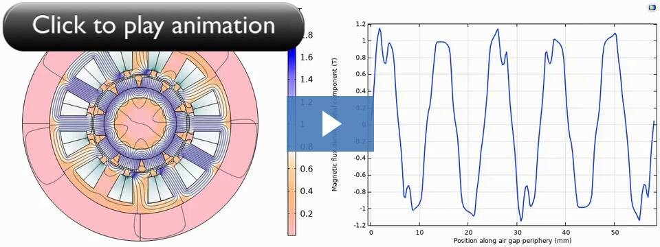
Left: Magnetic flux density variation with rotor rotation. Right: Progression of the air gap MMF wave with rotor rotation.
Investigating and Optimizing the Mechanical Torque
There are several ways to excite the stator windings for a particular slot/pole combination of a PM motor. The pattern shown in the schematic of the permanent magnet machine model (the first figure in the blog post) is one way in which a 12-slot, 10-pole PM motor can be driven. The stator coil excitation (or the initial rotor position) needs to be adjusted such that a maximum amount of torque is applied to the rotor. In order to do so, the rotor is given an initial angular displacement. The rotor angle is varied over an angular span of one rotor magnet, and the average torque is calculated. The value of initial angular displacement that corresponds to the maximum average torque is chosen as the initial position of the rotor. In this manner, it becomes easier to visualize what relative position of the stator and rotor produces maximum torque.
In the case presented here, two maxima are observed:
- Positive maximum that will correspond to a rotation in the counter-clockwise direction — once a proper phase sequence is applied.
- Negative maximum that will result in a clockwise rotation (also here, after fine-tuning the phase sequence)
The rotor torque waveform given in the next section corresponds to the positive maximum of the average rotor torque curve. We will look deeper into torque inspection and various methods of torque computation, such as Arkkio’s method and the virtual work principle, in upcoming blog posts.
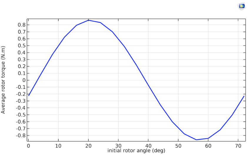
Variation of the average rotor torque with the initial rotor angle over the span of two rotor poles ().
Investigating and Optimizing the Iron Usage and the Losses
By using a magnetic flux density plot, we can investigate the flux density distribution in the iron core. In some portions of the geometry, the yoke may form a bottleneck, which may push the magnetic flux density value into the saturation region of the B-H curve. In others, it is wide enough to cause regions of low field intensity. When a certain part of the yoke consistently shows a weak field, that part is underutilized for torque production. When a certain part forms a consistent bottleneck, that part should probably be widened.
In the example, the iron thickness in the rotor and stator is varied, and its effect on the rotor torque is examined. For generating a maximum amount of torque, the initial rotor angle is set to , as obtained from the average torque curve in the previous section. As you can see from the plots and the torque curve below, the iron utilization is optimal when the iron thickness is about 2 mm: Going for less than 2 mm will have a negative effect on the torque, and going for more will add unnecessary material — and therefore; weight and cost — to the motor.
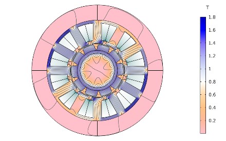
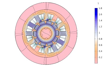
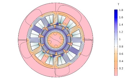
Magnetic flux density distribution for different values of iron thickness. Left: 1 mm. Center: 2 mm. Right: 3 mm.
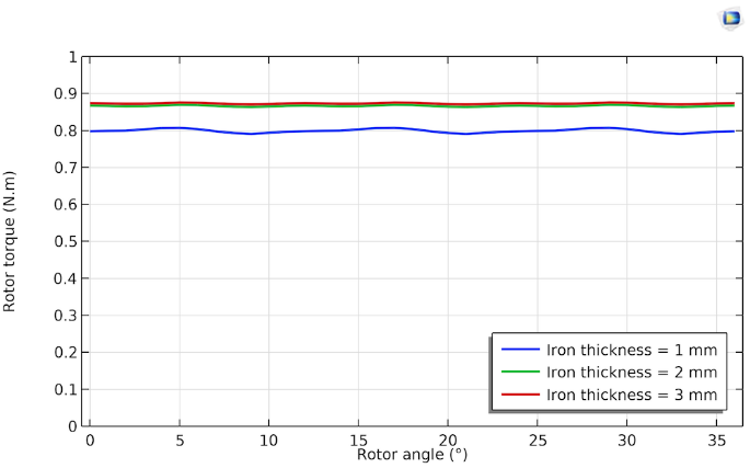
Rotor torque waveform variation with iron thickness
This isn’t the whole story though: There are additional considerations when determining the iron thickness, such as the mechanical strength and resistive and magnetic losses. When doing the investigation on the flux density and torque, the effect of the varying iron thickness on the iron losses can be evaluated as well. As of COMSOL Multiphysics version 5.6, there is a built-in Loss Calculation feature to easily assess the copper losses and iron losses using the Steinmetz equation, Bertotti formulation, or a user-defined loss model. In upcoming blog posts, we will further discuss the multiphysics aspects of rotating machine modeling, such as efficiency calculation, temperature rise assessment, vibration analysis, and noise examination.
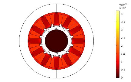
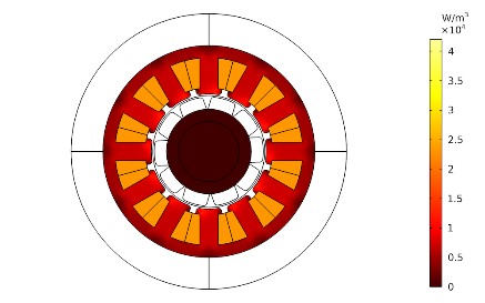
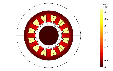
Iron loss distribution for different values of iron thickness. Left: 1 mm. Center: 2 mm. Right: 3 mm.
Summary
We have discussed the use of some functionality provided by Comsol Multiphysics and the AC/DC Module to easily get insights into a few design aspects of rotating machines. We have seen how the line graph of the radial magnetic flux density in the air gap shows us whether the induced voltage will be sinusoidal. Using Comsol Multiphysics, a Parametric Sweep can be used to determine the initial rotor angle that will produce the maximum rotor torque. The surface plot of the magnetic flux density in the machine enables you to visually determine whether the utilization of the iron is optimal for efficient torque production. The effect of the iron thickness on the iron losses can be observed as well, using the built-in loss models offered by COMSOL Multiphysics.
This first blog post in the series illustrates how the powerful modeling and post processing capabilities of COMSOL Multiphysics can be used to gain valuable insights into rotating machine design. The blog posts that follow will extensively discuss torque computation methods, efficiency calculation, analysis of iron losses and thermal performance, and motor vibration and noise examination.