Typically Testing Typical

Circular Logic

“Is this a riddle?” you say. No. This title sounds like it is circling, real circular logic, but it makes a point. Typical (typ) is typically the most misunderstood word in integrated circuit (IC) testing. There are other words to describe its concept: representative, emblematic, usual, normal, standard, mainstream, average, mean, and conventional. Confused? In the world of ICs, typical is defined as having the characteristics of the group of parts. Fine but, as the old English adage goes, that is as “clear as mud.”1 Let’s tell a sly secret of IC testing: typical on an IC data sheet means NOT TESTED. There, the secret is out. So why do IC manufacturers bother to state typical values? Let me explain.

Typical Values and a Range of Variety

Typical IC values cannot be tested directly because they are a statistical value. For example, it is like saying the average height of a human adult is 5 feet 5 inches. Measuring any single person will not allow you to establish a mean, an average, or a typical height. An anthropologist could measure the height of every race of mankind or statistically measure a sample of the population. Then a statistician, knowing the size of the sample, could calculate the confidence level of the average. This process is statistically the same for ICs. An IC designer can statistically predict a typical value based on simulation test results. Once again, typical is meant to give general guidance to the circuit designer.

IC data sheets generally list specifications in several categories:

• Absolute Maximum means do not exceed or the part may break.
• Electrical Characteristics are general conditions of test unless otherwise noted.
• Minimum (min), Typical (typ), and Maximum (max) specifications are measurements with specified units and conditions. Note that the “conditions” are the “unless otherwise noted” modifications
• Notes modify, limit, and clarify what is tested and how tests are preformed.

It will help to look at a common example. The following are general rules taken from a variety of data sheets from different IC manufacturers.

Min and max values are tested, unless otherwise noted, as specified under the Electrical Characteristics general conditions. You might see “TA = TMIN to TMAX, unless otherwise noted. Typical values are at TA = +25°C.” This means that the ambient temperature (TA) is equal to the temperature min and max listed for the operating temperature, unless the manufacturer says something different. Typical values are at TA = +25°C only. Notes follow, and the common ones are:

Note 1: All devices are 100% production tested at +25°C and are guaranteed by design for TA = TMIN to TMAX, as specified.

Note 2: Linearity is tested within 20mV of GND and AVDD, allowing for gain and offset error.

Note 3: Codes above 2047 are guaranteed to be within ±8 LSB (least significant bit).

Note 4: Gain and offset are tested within 100mV of GND and AVDD.

Note 5: Guaranteed by design.

The end of Note 1 and Note 5 say “guaranteed by design.” This deserves more explanation. All IC fabrication (fab) processes have variations. Because the components and multiple layers are so small, almost anything causes changes. These deviations are the normal range of variety.

We will explain these notes using a section of a MAX5134 to MAX5137 data sheet (Figure 1).

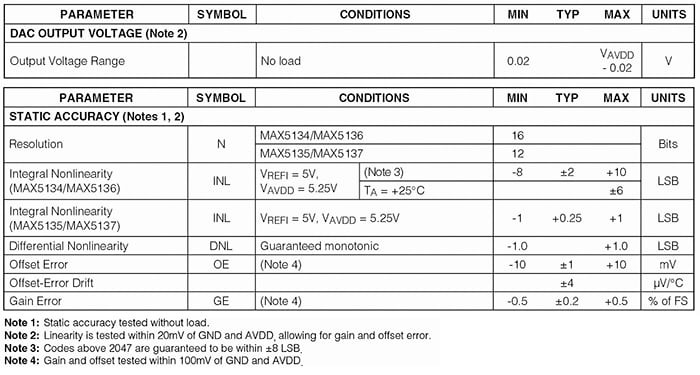
Figure 1: Values from a MAX5134 to Max5137 Digital-to-Analog Converter (DAC) family data sheet.

Notes 2 and 4 are common for rail-to-rail op amps and buffered-output DACs. Observe that the Output Voltage Range is cataloged with the condition of “No load.” This is because the so-called rail-to-rail operation is, quite honestly, wishful thinking. It is not perfect, but certainly much better than older devices with output circuits that started running out of current a volt from the voltage rails.

Note 3 is common for DACs. Codes below a number near the bottom (usually ground) and above a number near the top voltage rail are not as linear as the center codes. Here the bottom 2047 codes out of the 65,536 total have an INL (integral nonlinearity) of ±10 LSBs; above 2047, the INL is only ±8 LSBs.

Let’s digress for a moment. Think about buying paint for your home. The home center encourages you to bring in a swatch of cloth so they can exactly match its color on their color-matching machine. Then they take a white base paint and the machine automatically adds multiple pigments to get the “exact matching color.” This process is repeated for each can of paint purchased. After all this exact matching, what do they tell you to do? What does a professional painter do? Take all the cans of paint and mix them together. Why? The human eye and brain can compare colors with more precision and can thus see any residual color errors from different mixes on the “exact matching” machine. This is not entirely the machine’s fault. The mixing machine’s metering valves, the color-separation filters, the calibration of gain and offset are not perfect. The pigments themselves even have an acceptable range of color and viscosity. The paint process goes on and on with tolerances adding, combining, and sometimes multiplying to produce small but visible errors—the range of variety, the standard deviations.

Figure 2 is a commonly accepted standard-deviation or bell curve. The solid dark line represents the normal distribution that we would like to see. The green dotted line shows that the process is moved to right of center— hopefully we understand what caused this deviation so we can correct it. The long dashed blue line is a bifurcated curve which could be two parameters moving. More complex curves result when many different factors can change. This is why professional painters mix the cans together before applying the paint to the wall. Isn’t averaging errors wonderful?

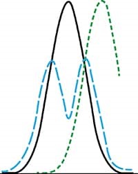
Figure 2: A process standard-deviation or bell curve. The more factors that are changing, the more complex the curve.

Compensating for Process Variations

To ensure that an IC will meet its specifications, several layers of engineering safety factors are designed into the IC fabrication process to average away possible errors. No engineering group wants to ship “out of specification” parts. Consequently, the designers leave ample leeway with part specifications, and then the test and QA engineers expect “six sigma limits” for the expected variations. The resulting performance specifications are very conservative.

The design process compensates for many design, manufacturing and process differences. Therefore, designers use simulation tools to explore the fab process variation “corners.” The reasoning is straightforward. If they worry about the corners, then the center of the process will be fine. They then modify the circuits to make them as immune as is reasonable to those process corners. The most extreme corners are hot-fast and cold-slow (see Figure 3). Hot and cold are temperatures. Fast is high gain, high electron mobility; slow is the opposite. Designers can optimize to the design criteria, but cannot optimize everything. Consequently, parameters that are not specified will not be addressed.

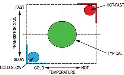
Figure 3: IC process fab variations.

Understanding Six Sigma

Six sigma2 was originally developed by Bill Smith at Motorola in 1986 as a set of practices designed to improve manufacturing processes and eliminate defects. Sigma (the lower-case Greek letter s) is used to represent the standard deviation (i.e., a measure of variation) of a statistical population. The term “six sigma process” comes from the premise that if one has six standard deviations between the mean of a process and the nearest specification limit, then there will be practically no items that fail to meet the specifications. This conclusion is based on the calculation method employed in a process capability study.

In a capability study, the number of standard deviations between the process mean and the nearest specification limit is given in sigma units. As process standard deviation rises, or as the mean of the process moves away from the center of the tolerance, fewer standard deviations will fit between the mean and the nearest specification limit. This decreases the sigma number.

The Role of the 1.5 Sigma Shift

Experience has shown that, in the long term, processes usually do not perform as well as they do in the short term. Consequently, the number of sigmas that will fit between the process mean and the nearest specification limit is likely to drop over time. This has proven true when compared to an initial short-term study. To account for this real-life increase in process variation over time, an empirically-based 1.5 sigma shift is introduced into the calculation. According to this premise, a process that fits six sigmas between the process mean and the nearest specification limit in a short-term study will in the long term only fit 4.5 sigmas. This happens because either the process mean will move over time, or the long-term standard deviation of the process will be greater than that observed in the short term, or both.

Hence, the widely accepted definition of a six sigma process is one that produces 3.4 defective parts per million opportunities (DPMO). This definition is based on the fact that a process that is normally distributed will have 3.4 parts per million beyond a point that is 4.5 standard deviations above, or below, the mean. (This is a one-sided capability study.) So the 3.4 DPMO of a six sigma process effectively corresponds to 4.5 sigmas, namely six sigmas, minus the 1.5 sigma shift introduced to account for long-term variation. This theory is designed to prevent underestimating the defect levels likely to be encountered in real-life operation.

When taking the 1.5 sigma shift into account, the short-term sigma levels correspond to the following long-term DPMO values (one-sided).

• One sigma = 690,000 DPMO = 31% efficiency
• Two sigmas = 308,000 DPMO = 69.2% efficiency
• Three sigmas = 66,800 DPMO = 93.32% efficiency
• Four sigmas = 6,210 DPMO = 99.379% efficiency
• Five sigmas = 230 DPMO = 99.977% efficiency
• Six sigmas = 3.4 DPMO = 99.9997% efficiency

Conclusion

We trust that the above discussion helps to explain the reasons behind the fab testing and how typical values are really typical (i.e., normal).

Now let’s carry this a step further. Suppose that we want to design a measuring instrument that will be used in a testing laboratory environment. To set instrument specifications, we need to understand and control component manufacturing variations. Knowing that the ICs we use are six-sigma accurate helps us to have confidence in our final instrument specifications. Here we added that the instrument will operate at room temperature. You might have missed that, but above we specified a “testing laboratory environment”. This is a key specification. If this instrument is for field use, one must explicitly specify the temperature, humidity, and atmospheric pressure for the particular field of operation. For medical use, we must answer what patient-specific portion needs to be sterilized or disposable. If the instrument can be used in space or on a rocket, what vibration, atmospheric pressure, radiation hardness, temperature endurance are required?

In short, knowing that we are starting with six-sigma ICs will give us “typical confidence” in the typical guidance provided by the IC data sheet.