


Walter Frei, Comsol
If you are modeling electrical signals that are varying arbitrarily in time, you can often use the computationally efficient Electric Currents interface in the COMSOL Multiphysics software to compute the response of the system via a time-dependent study. Although there are several different excitation options, we will usually want to think in terms of either an applied current signal or a voltage signal traveling along a transmission line. Let’s take a deeper look at why this is.


Introduction
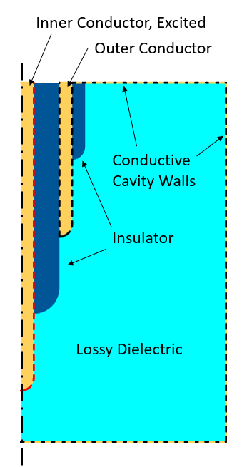
Here, we will look at the example used in our previous blog post, “Using Different Physics Interfaces for RF Electromagnetic Heating Models”: frequency-domain excitations of a coaxial cable inserted into a metal cavity filled with a sample of lossy dielectric material. We will use the same system and apply various types of transient signals to the coax as well as compare the Electric Currents physics interface with the Electromagnetic Waves, Transient physics interface, primarily in terms of computing the total dissipation within the material. The reason for comparing these two interfaces is that the Electromagnetic Waves, Transient interface solves the full vectorial form of Maxwell’s equations, whereas the Electric Currents interface solves for a simplified approximation of Maxwell’s equations by ignoring the magnetic fields and solving solely for the scalar electric potential. To reduce the computational cost of these examples, the model will be reduced to the 2D axisymmetric modeling plane, as shown in the schematic below.
Current Excitation
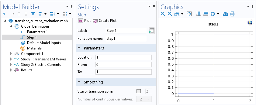
We begin with exciting the system via a prescribed current, with a variation in time, as shown in the figure below. The signal is initially zero, and then steps up to a maximum value, which is then maintained. It’s possible to apply smoothing to this step function, which will be considered later. The system starts in its unexcited state: the fields are initially zero everywhere. Given this initial condition and input signal, the transient system response should approach a nonzero steady-state solution after sufficient time, equivalent to a DC excitation of the system.
We will first build a model using the Electromagnetic Waves, Transient interface since this interface captures all resistive, capacitive, and inductive phenomena. This interface is different from the Electromagnetic Waves, Frequency Domain interface used previously, in that it does not include an Impedance Boundary Condition, as this boundary condition only has meaning in the frequency domain. Although it’s possible to explicitly model the metal leads, we will instead model all metallic parts as lossless, ideal conductors via the Perfect Electric Conductor boundary condition. This is justified, as it was previously shown that the losses in the metal are relatively negligible for this case.
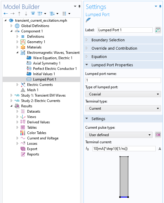
We use the Lumped Port boundary condition, of type Coaxial, and specify a transient applied current. Note that the argument to the Step function is entered in nondimensionalized units. The total simulated timespan is 150 ns, with results saved every 1 ns. The plot below shows the voltage sensed at the Lumped Port boundary condition (within the Electromagnetic Waves, Transient interface, which is abbreviated as TEMW in the figure below). The curve shows the typical response we should expect from a resistive–capacitive system.

The same situation is modeled with the Electric Currents interface, which considers only resistive and capacitive effects. In this interface, the Terminal boundary condition of type Current will inject the specified current at the inner conductor. The outer conductor and remaining exterior boundaries are all set to Ground. To compare solutions, the maximum solver time step is also set to 1 ns, and the results show excellent agreement.
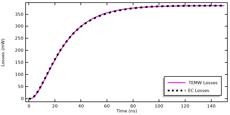
This plot shows a comparison of the deposited heat into the model over time for both physics’ interfaces, and shows agreement. We can also compute the integrated losses over time via the timeint() operator, which has the following syntax:
timeint(0,150e-9, intopSample(ec.Qh), ‘nointerp’),
where the added ‘nointerp’ option evaluates the time integral of the integration over the volume using solely the saved time steps, and both interfaces compute a total deposited energy of 46.8 nJ over this 0– 150 ns timespan, with less than a 1% difference. Based on this data, it’s possible to conclude that, for this system excited by this current signal, the Electric Currents interface will give nearly identical results as the Electromagnetic Waves, Transient interface, and at lower computational cost.
Voltage Excitations in Electric Currents
Next, let’s use the same step function but instead use it to modulate the Terminal Voltage within the Electric Currents interface. That is, we will try to instantly change the applied voltage between the inner and outer conductor of the coaxial cable. We can try to solve such a model, but it will actually lead to a solver failure. This should not be too surprising, since a capacitive device resists an instantaneous change in voltage. That is, the step input to the voltage is nonphysical.
Instead of trying to solve such a nonphysical excitation, we can go back to the Step function and enable smoothing. With this change, we can solve the model over a shorter timespan of 5 ns, with results saved every 0.01 ns, and with a tighter solver relative tolerance of 1e-5, as described in our “Controlling the Time-Dependent Solver Timesteps” knowledge base entry.
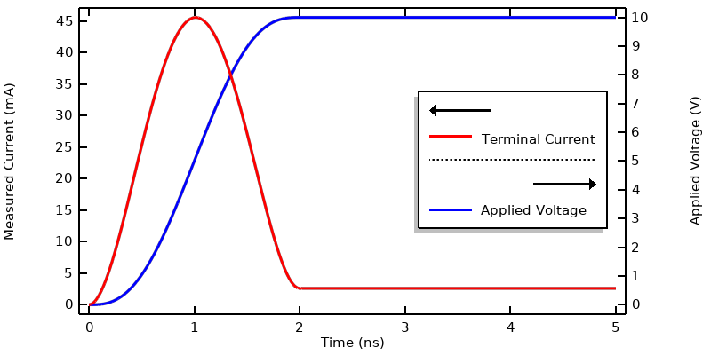
This figure shows the applied voltage and the current through the terminal. Note that the current rises to over ten times the steady-state current as the applied voltage is rising. To understand this, examine the expression for the current, as defined within the Electric Currents interface:
![]()
This is the sum of the conduction current and displacement current, and the electric field is computed from ![]() . So, if the electric potential as a function of time is specified at a boundary, then both the conduction current and the displacement current into the model are specified, and that is nonphysical. Contrast this with the previous case of an applied current, where only the total current is specified, and the model computes what fraction of that total current is displacement current or conduction current.
. So, if the electric potential as a function of time is specified at a boundary, then both the conduction current and the displacement current into the model are specified, and that is nonphysical. Contrast this with the previous case of an applied current, where only the total current is specified, and the model computes what fraction of that total current is displacement current or conduction current.
We should also ask if it’s possible to apply an analogous boundary condition in the Electromagnetic Waves, Transient interface. This is not possible; this interface uses the magnetic vector potential formulation, which does not admit such an excitation condition. Even if it was possible via the numerical method, this type of excitation is not physically plausible since it would imply a kind of feedback control problem.
It’s still valid to use the voltage excitation in the Electric Currents interface in the time domain, but only in those specific cases where the resultant displacement current at the terminal boundary is relatively much smaller than the conduction current. That is, use the voltage boundary condition only for those cases where the device is almost purely resistive. The case we’re looking at here, though, requires that we look to a more realistic boundary condition.
Transmission Lines, Lumped Ports, and Terminated Terminal Conditions
Within the Electromagnetic Waves, Transient interface, let’s now take another look at the Lumped Port boundary condition. The Current type was already discussed, and the Circuit type will be discussed later, so we will now focus on the Cable type. The Cable option presents the ability to define a voltage signal and a cable impedance. This gives us a condition that can be understood in the context of an infinite lossless transmission line of specified impedance, for example ![]() , with a source placed along the infinite cable. This source imposes a current such that a signal propagates in both directions along the transmission line away from the source, and such that the sensed voltage will be equal to the defined signal. Since the signal propagates in both directions, the magnitude of this imposed current is
, with a source placed along the infinite cable. This source imposes a current such that a signal propagates in both directions along the transmission line away from the source, and such that the sensed voltage will be equal to the defined signal. Since the signal propagates in both directions, the magnitude of this imposed current is ![]() This is based on the specified voltage signal, V(t), and the specified cable impedance — assuming that the system impedance matches the cable impedance. In actuality, the cable impedance will be different from the system impedance, Zs, so the signal will be partially reflected by the system model and back into the transmission line. So, the input signal is entered at this boundary in terms of voltage, but in actuality imposes a fixed current as well as a parallel load equal to the cable impedance. We can think of the signal coming from the current source as being split into the cable and system, with some fraction of that signal reflected back. In most real sources, there would be some kind of circulator or isolator that would prevent the reflected signal from interacting with the current source, and divert the reflected signal to a matched dissipative load.
This is based on the specified voltage signal, V(t), and the specified cable impedance — assuming that the system impedance matches the cable impedance. In actuality, the cable impedance will be different from the system impedance, Zs, so the signal will be partially reflected by the system model and back into the transmission line. So, the input signal is entered at this boundary in terms of voltage, but in actuality imposes a fixed current as well as a parallel load equal to the cable impedance. We can think of the signal coming from the current source as being split into the cable and system, with some fraction of that signal reflected back. In most real sources, there would be some kind of circulator or isolator that would prevent the reflected signal from interacting with the current source, and divert the reflected signal to a matched dissipative load.
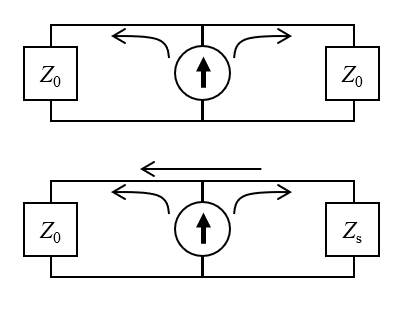
The circuit equivalent interpretation of the Lumped Port boundary condition, of type Cable. The top figure shows the assumed case: The signal propagates from the current source into the cable and system, of matched impedance. The source sits within the cable, so the signal propagates in both directions. The bottom figure shows the modeled case: The mismatched impedance of the system leads to a fraction of the signal being reflected back into the cable.
The analogous boundary condition within the Electric Currents interface is the Terminal condition of type Terminated. Here, we can similarly input a cable impedance, but instead need to apply a power, rather than voltage, where the power is ![]() .
.
The model can be solved using finer output time steps and tolerances for both physics. The results can be evaluated in terms of measured voltage and current as well as losses and integrated losses over time, as shown below. There are several features to remark on:
- The sensed voltage and current from the Electromagnetic Waves, Transient interface shows ripples, or waves, in the signal. This is expected. These ripples are due to the frequency content of the input signal and also arise due to reflections of the signal from the materials, boundary conditions, and geometry of the system model.
- The sensed voltage is nearly twice the applied voltage. This is due to the fact that this boundary condition can also be thought of as a Norton equivalent of a voltage source, but with a Norton resistance equal to the cable impedance, which, in this case, is relatively small compared to the resistance of the system being modeled.
- The solution from the Electric Currents interface does not have any ripples since this interface explicitly ignores the inductive effects, but the overall shape is very similar and gives the same steady-state solution.
- The losses agree well, and the total deposited energy agrees to within 1%.
We can thus conclude that the Electric Currents interface is a very good approximation of the full Electromagnetic Waves, Transient interface, for this system and excitation type.
Plot of measured voltage and measured current when modeling an applied smoothed step voltage signal propagating along a transmission line.
Comparison of computed losses with the sample material when a smoothed step voltage signal is applied.
Electrical Circuit Connections
Looking at the circuit diagram in the previous figure, it appears as if the Lumped Port, of type Cable, represents a resistor attached to the system. We could check this interpretation by instead using the Lumped Port, of type Circuit, and adding a lumped current source and a lumped resistor in parallel with the system via the Electrical Circuits interface. The approach of connecting these physics interfaces is similar to what was shown in our blog post “Understanding the Excitation Options for Modeling Electric Currents”. This same excitation can be reproduced by connecting the Electric Currents interface to the Electrical Circuits interface via the Terminal condition of type Circuit.
A more complex matching circuit, including capacitors, inductors, and transformers, could also be implemented in the Electrical Circuit interface. It can be reasonable to use a voltage source feature within the Electrical Circuits interface as long as the additional elements are added to the circuit to prevent any kind of nonphysical excitation. Nonlinear lumped devices, diodes and transistors, can also be included, although these will result in a set of equations that are more computationally intensive to solve, and might require further modification of solver settings.
A Quick Word About Deposited Power
Looking back on the blog post about frequency-domain excitations of this system, we also implemented an excitation that would deposit a known power into the system. This type of excitation is based on feedback, meaning that it monitors some state of the model and feeds information back to the input. Such feedback is reasonable in a frequency-domain model, under the implicit assumption that the feedback happens over several cycles. It’s much less motivated for a time-domain model, where any feedback would also have to include the dynamics and delay of the control system. Such time-domain feedback is not motivated for systems and timespans similar to what we have looked at here.
Closing Remarks
We’ve looked at various ways of exciting a system with a time-domain signal within both the Electric Currents interface and the Electromagnetic Waves, Transient interface. For the particular system and the signal that was being considered, these two interfaces produce very similar results. The Electric Currents interface is appropriate when the electric energy in the excited system is much greater than the magnetic energy. The alternate case, when the system is primarily inductive and the magnetic fields are much greater than the electric fields, will be looked at separately in a future blog post.
We have seen that all excitations are fundamentally specifying the current going into the system model. The case of a voltage signal propagating along a transmission line is simply a Norton equivalent: a current source with an external resistance — representing the transmission line — parallel to the system model. Ultimately, the choice between these excitation options representing a current source, a voltage signal propagating along a transmission line, or adding an Electrical Circuit interface depends on the type of source that you are working with.
The signals that have been looked at here are quite simple, but we often need to consider more complicated transient signals, and especially signals that are periodic. Such signals lend themselves to some very efficient modeling techniques, which will be addressed in a following article, so stay tuned!