


Motivation
3D reconstruction is a long-standing problem in computer vision, with applications in robotics, VR and multimedia. It is a notorious problem since it requires lifting 2D images to 3D space in a dense, accurate manner.
Gaussian splatting (GS) [1] represents 3D scenes using volumetric splats, which can capture detailed geometry and appearance information. It has become quite popular due to their relatively fast training, inference speeds and high quality reconstruction.


GS-based reconstructions generally consist of millions of Gaussians, which makes them hard to use on computationally constrained devices such as smartphones. Our goal is to improve storage and computational inefficiency of GS methods. Hence, we propose Trick-GS, a set of optimizations that enhance the efficiency of Gaussian Splatting without significantly compromising rendering quality.
Background
GS is a method for representing 3D scenes using volumetric splats, which can capture detailed geometry and appearance information. It has become quite popular due to their relatively fast training, inference speeds and high quality reconstruction.
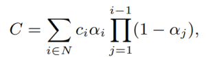
GS reconstructs a scene by fitting a collection of 3D Gaussian primitives, which can be efficiently rendered in a differentiable volume splatting rasterizer by extending EWA volume splatting [2]. A scene represented with 3DGS typically consists of hundreds of thousands to millions of Gaussians, where each 3D Gaussian primitive consists of 59 parameters. The technique includes rasterizing Gaussians from 3D to 2D and optimizing the Gaussian parameters where a 3D covariance matrix of Gaussians are later parameterized using a scaling matrix and a rotation matrix. Each Gaussian primitive also has an opacity (α ∈ [0, 1]), a diffused color and a set of spherical harmonics (SH) coefficients, typically consisting of 3-bands, to represent view-dependent colors. Color C of each pixel in the image plane is later determined by Gaussians contributing to that pixel with blending the colors in a sorted order.
GS initializes the scene and its Gaussians with point clouds from SfM based methods such as Colmap. Later Gaussians are optimized and the scene structure is changed by removing, keeping or adding Gaussians to the scene based on gradients of Gaussians in the optimization stage. GS greedily adds Gaussians to the scene and this makes the approach in efficient in terms of storage and computation time during training.
Tricks for Learning Efficient 3DGS Representations
We adopt several strategies that can overcome the inefficiency of representing the scenes with millions of Gaussians. Our adopted strategies mutually work in harmony and improve the efficiency in different aspects. We mainly categorize our adopted strategies in four groups:
a) Pruning Gaussians; tackling the number of Gaussians by pruning.
b) SH masking; learning to mask less useful Gaussian parameters with SH masking to lower the storage requirements.
c) Progressive training strategies; changing the input representation by progressive training strategies.
d) Accelerated implementation; the optimization in terms of implementation.
a) Pruning Gaussians:
a.1) Volume Masking
Gaussians with low scale tend to have minimal impact on the overall quality, therefore we adopt a strategy that learns to mask and remove such Gaussians. N binary masks, M ∈ {0, 1}N , are learned for N Gaussians and applied on its opacity, α ∈ [0, 1]N , and non-negative scale attributes, s by introducing a mask parameter, m ∈ RN. The learned masks are then thresholded to generate hard masks M;
![]()
These Gaussians are pruned at densification stage using these masks and are also pruned at every km iteration after densification stage.
a.2) Significance of Gaussians
Significance score calculation aims to find Gaussians that have no impact or little overall impact. We adopt a strategy where the impact of a Gaussian is determined by considering how often it is hit by a ray. More concretely, the so called significance score GSj is calculated with 1(G(Xj ), ri) where 1(·) is the indicator function, ri is ray i for every ray in the training set and Xj is the times Gaussian j hit ri.
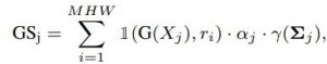
where j is the Gaussian index, i is the pixel, γ(Σj ) is the Gaussian’s volume, M, H, and W represents the number of training views, image height, and width, respectively. Since it is a costly operation, we apply this pruning ksg times during training with a decay factor considering the percentile removed in the previous round.
b) Spherical Harmonic (SH) Masking
SHs are used to represent view dependent color for a Gaussian, however, one can appreciate that not all Gaussians will have the same levels of varying colors depending on the scene, which provides a further pruning opportunity. We adopt a strategy where SH bands are pruned based on a mask learned during training, and unnecessary bands are removed after the training is complete. Specifically, each Gaussian learns a mask per SH band. SH masks are calculated as in the following equation and SH values for the ith Gaussian for the corresponding SH band, l, is set to zero if its hard mask, Mshi(l), value is zero and unchanged otherwise.
![]()
where mli ∈ (0, 1), Mlsh ∈ {0, 1}. Finally, each masked view dependent color is defined as ĉi(l) = Mshi(l)ci(l) where ci(l) ∈ R(2l+1)×3. Masking loss for each degree of SH is weighted by its number of coefficients, since the number of SH coefficients vary per SH band.
c) Progressive training strategies
Progressive training of Gaussians refers to starting from a coarser, less detailed image representation and gradually changing the representation back to the original image. These strategies work as a regularization scheme.
c.1) By blurring
Gaussian blurring is used to change the level of details in an image similar. Kernel size is progressively lowered at every kb iteration based on a decay factor. This strategy helps to remove floating artifacts from the sub-optimal initialization of Gaussians and serves as a regularization to converge to a better local minima. It also significantly impacts the training time since a coarser scene representation requires less number of Gaussians to represent the scene.
c.2) By resolution
Progressive training by resolution. Another strategy to mitigate the over-fitting on training data is to start with smaller images and progressively increase the image resolution during training to help learning a broader global information. This approach specifically helps to learn finer grained details for pixels behind the foreground objects.
c.3) By scales of Gaussians
Another strategy is to focus on low-frequency details during the early stages of the training by controlling the low-pass filter in the rasterization stage. Some Gaussians might become smaller than a single pixel if each 3D Gaussian is projected into 2D, which results in artefacts. Therefore, the covariance matrix of each Gaussian is added by a small value to the diagonal element to constraint the scale of each Gaussian. We progressively change scale for each Gaussian during the optimization similar to ensure the minimum area that each Gaussian covers in the screen space. Using a larger scale in the beginning of the optimization enables Gaussians receive gradients from a wider area and therefore the coarse structure of the scene is learned efficiently.
d) Accelerated Implementation
We adopt a strategy that is more focused on the training time efficiency. We follow on separating higher SH bands from the 0th band within the rasterization, thus lower the number of updates for the higher SH bands than the diffused colors. SH bands (45 dims) cover a large proportion of these updates, where they are only used to represent view-dependent color variations. By modifying the rasterizer to split SH bands from the diffused color, we update higher SH bands every 16 iterations whereas diffused colors are updated at every iteration.
GS uses photometric and structural losses for optimization where structural loss calculation is costly. SSIM loss calculation with optimized CUDA kernels. SSIM is configured to use 11×11 Gaussian kernel convolutions by standard, where as an optimized version is obtained by replacing the larger 2D kernel with two smaller 1D Gaussian kernels. Applying less number of updates for higher SH bands and optimizing the SSIM loss calculation have a negligible impact on the accuracy, while it significantly helps to speed-up the training time as shown by our experiments.
Experimental Results
We follow the setup on real-world scenes. 15 scenes from bounded and unbounded indoor/outdoor scenarios; nine from Mip-NeRF 360, two (truck and train) from Tanks&Temples and two (DrJohnson and Playroom) from Deep Blending datasets are used. SfM points and camera poses are used as provided by the authors [1] and every 8th image in each dataset is used for testing. Models are trained for 30K iterations and PSNR, SSIM and LPIPS are used for evaluation. We save the Gaussian parameters in 16-bit precision to save extra disk space as we do not observe any accuracy drop compared to 32-bit precision.
Performance Evaluation
Our most efficient model Trick-GS-small improves over the vanilla 3DGS by compressing the model size drastically, 23×, improving the training time and FPS by 1.7× and 2×, respectively on three datasets. However, this results in slight loss of accuracy, and therefore we use late densification and progressive scale-based training with our most accurate model Trick-GS, which is still more efficient than others while not sacrificing on the accuracy.

Table 1. Quantitative evaluation on MipNeRF 360 and Tanks&Temples datasets. Results with marked ’∗’ method names are taken from the corresponding papers. Results between the double horizontal lines are from retraining the models on our system. We color the results with 1st, 2nd and 3rd rankings in the order of solid to transparent colored cells for each column. Trick-GS can reconstruct scenes with much lower training time and disk space requirements while not sacrificing on the accuracy.
Trick-GS improves PSNR by 0.2dB on average while losing 50% on the storage space and 15% on the training time compared to Trick-GS-small. The reduction on the efficiency with Trick-GS is because of the use of progressive scale-based training and late densification that compensates for the loss from pruning of false positive Gaussians. We tested an existing post-processing step, which helps to further reduce model size as low as 6MB and 12MB respectively for Trick-GS-small and Trick-GS over MipNeRF 360 dataset. The post-processing does not heavily impact the training time but the accuracy drop on PSNR metric is 0.33dB which is undesirable for our method. Thanks to our trick choices, Trick-GS learns models as low as 10MB for some outdoor scenes while keeping the training time around 10mins for most scenes.
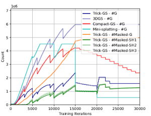
Figure 1. Number of Gaussians (#G) during training (on MipNeRF 360 – bicycle scene) for all methods, number of masked Gaussians (#Masked-G) and number of Gaussians with a masked SH band for our method. Our method performs a balanced reconstruction in terms of training efficiency by not letting the number of Gaussians increase drastically as other methods during training, which is a desirable property for end devices with low memory.
Learning to mask SH bands helps our approach to lower the storage space requirements. Trick-GS lowers the storage requirements for each scene over three datasets even though it might result in more Gaussians than Mini-Splatting for some scenes. Our method improves some accuracy metrics over 3DGS while the accuracy changes are negligible. Advantage of our method is the requirement of 23× less storage and 1.7× less training time compared to 3DGS. Our approach achieves this performance without increasing the maximum number of Gaussians as high as the compared methods. Fig. 1 shows the change in number of Gaussians during training and an analysis on the number of pruned Gaussians based on the learned masks. Trick-GS achieves comparable accuracy level while using 4.5× less Gaussians compared to Mini-Splatting and 2× less Gaussians compared to Compact-GS, which is important for the maximum GPU consumption on end devices. Fig. 2 shows the qualitative impact of our progressive training strategies. Trick-GS obtains structurally more consistent reconstructions of tree branches thanks to the progressive training.
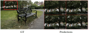
Figure 2. Impact of progressive training strategies on challenging background reconstructions. We empirically found that progressive training strategies as downsampling, adding Gaussian noise and changing the scale of learned Gaussians have a significant impact on the background objects with holes such as tree branches.
Ablation Study
We evaluate the contribution of tricks in Tab. 2 on MipNeRF360 – bicycle scene. Our tricks mutually benefits from each other to enable on-device learning. While Gaussian blurring helps to prune almost half of the Gaussians compared to 3DGS with a negligible accuracy loss, downsampling the image resolution helps to focus on the details by the progressive training and hence their mixture model lowers the training time and the Gaussian count by half. Significance score based pruning strategy improves the storage space the most among other tricks while masking Gaussians strategy results in lower number of Gaussians at its peak and at the end of learning. Enabling progressive Gaussian scale based training also helps to improve the accuracy thanks to having higher number of Gaussians with the introduced split strategy.
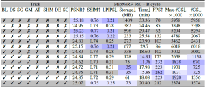
Table 2. Ablation study on tricks adopted by our approach using‘bicycle’ scene. Our tricks are abbreviated as BL: progressive Gaussian blurring, DS: progressive downsampling, SG: significance pruning, GM: Gaussian masking, SHM: SH masking, AT: accelerated training, DE: late densification, SC: progressive scaling. Our full model Trick-GS uses all the tricks while Trick-GS-small uses all but DE and SC.
Summary and Future Directions
We have proposed a mixture of strategies adopted from the literature to obtain compact 3DGS representations. We have carefully designed and chosen strategies from the literature and showed competitive experimental results. Our approach reduces the training time for 3DGS by 1.7×, the storage requirement by 23×, increases the FPS by 2× while keeping the quality competitive with the baselines. The advantage of our method is being easily tunable w.r.t. the application/device needs and it further can be improved with a post-processing stage from the literature e.g. codebook learning, huffman encoding. We believe a dynamic and compact learning system is needed based on device requirements and therefore leave automatizing such systems for future work.